How do we describe movement mathematically?
Imagine that you are standing at the point $(0,0)$.
Someone tells you:
Move 3 units to the right and 2 units upward.
You could describe that movement with words.
But mathematics gives us a much more compact way:
\[\mathbf{v} = \begin{bmatrix} 3\\ 2 \end{bmatrix}\]This object is called a vector.
The two numbers tell us how much movement occurs in each direction.
The first component tells us the horizontal movement.
The second component tells us the vertical movement.
So
\[\mathbf{v} = \begin{bmatrix} 3\\ 2 \end{bmatrix}\]means:
- move $3$ units horizontally;
- move $2$ units vertically.
That simple idea is the beginning of linear algebra.
1. Seeing a vector
A vector can be represented geometrically as an arrow.
The arrow starts at the origin and points toward the location described by its components.
For
\[\mathbf{v} = \begin{bmatrix} 3\\ 2 \end{bmatrix},\]the arrow goes from
\[(0,0)\]to
\[(3,2).\]The arrow is not just a picture.
It is telling us something precise:
\[\boxed{ \mathbf{v} = \begin{bmatrix} 3\\ 2 \end{bmatrix}}\]The vector has a horizontal component of $3$ and a vertical component of $2$.
2. The components of a vector
Consider the vector
\[\mathbf{v} = \begin{bmatrix} a\\ b \end{bmatrix}.\]We call $a$ and $b$ the components of the vector.
For example,
\[\mathbf{v} = \begin{bmatrix} 5\\ -2 \end{bmatrix}\]has
\[\text{horizontal component}=5\]and
\[\text{vertical component}=-2.\]The negative sign tells us that the vertical movement is downward.
3. Vectors are not points
This distinction is important.
Suppose we have a point
\[P=(3,2).\]This tells us where something is.
But the vector
\[\mathbf{v} = \begin{bmatrix} 3\\ 2 \end{bmatrix}\]tells us how to move.
These ideas are related, but they are not exactly the same.
We can use a vector to move from one point to another.
Suppose
\[P=(1,1)\]and
\[\mathbf{v} = \begin{bmatrix} 3\\ 2 \end{bmatrix}.\]Adding the vector to the point gives
\[P+\mathbf{v} = (1,1)+(3,2) = (4,3).\]So the vector moves us from $(1,1)$ to $(4,3)$.
4. A vector can start anywhere
Here is another important idea.
Consider
\[\mathbf{v} = \begin{bmatrix} 3\\ 2 \end{bmatrix}.\]It does not have to start at the origin.
We could draw the same vector starting at
\[(1,1)\]and ending at
\[(4,3).\]The movement is still:
\[3\text{ units right}\]and
\[2\text{ units up}.\]So these two arrows represent the same vector:
\[(0,0)\rightarrow(3,2)\]and
\[(1,1)\rightarrow(4,3).\]The starting location changes, but the movement does not.
This is why we often think of vectors as free arrows.
5. Vectors can be added
Now suppose we make two movements.
The first movement is
\[\mathbf{u} = \begin{bmatrix} 3\\ 2 \end{bmatrix}.\]The second movement is
\[\mathbf{v} = \begin{bmatrix} 1\\ 4 \end{bmatrix}.\]Our total movement is
\[\mathbf{u}+\mathbf{v}.\]We add the corresponding components:
\[\mathbf{u}+\mathbf{v} = \begin{bmatrix} 3\\ 2 \end{bmatrix} + \begin{bmatrix} 1\\ 4 \end{bmatrix}\]and therefore
\[\mathbf{u}+\mathbf{v} = \begin{bmatrix} 4\\ 6 \end{bmatrix}\]So vector addition is simply component-by-component addition.
6. Scalar multiplication
Vectors can also be multiplied by ordinary numbers.
These numbers are called scalars.
Suppose
\[\mathbf{v} = \begin{bmatrix} 2\\ 1 \end{bmatrix}.\]Multiply it by $3$:
\[3\mathbf{v} = 3 \begin{bmatrix} 2\\ 1 \end{bmatrix}.\]Multiply each component by $3$:
\[3\mathbf{v} = \begin{bmatrix} 6\\ 3 \end{bmatrix}.\]Geometrically, the vector becomes three times as long.
In general,
\[c \begin{bmatrix} x\\ y \end{bmatrix} = \begin{bmatrix} cx\\ cy \end{bmatrix}.\]7. What if the scalar is negative?
Consider
\[\mathbf{v} = \begin{bmatrix} 2\\ 1 \end{bmatrix}.\]Multiplying by $-1$ gives
\[-\mathbf{v} = \begin{bmatrix} -2\\ -1 \end{bmatrix}.\]The vector now points in the opposite direction.
So:
\[\text{positive scalar} \rightarrow \text{same direction}\]while
\[\text{negative scalar} \rightarrow \text{opposite direction}\]This simple operation will become extremely important when we study linear combinations.
8. How long is a vector?
So far we have talked about the direction of a vector.
But a vector also has a magnitude — its length.
For
\[\mathbf{v} = \begin{bmatrix} 3\\ 4 \end{bmatrix},\]the horizontal and vertical components form a right triangle.
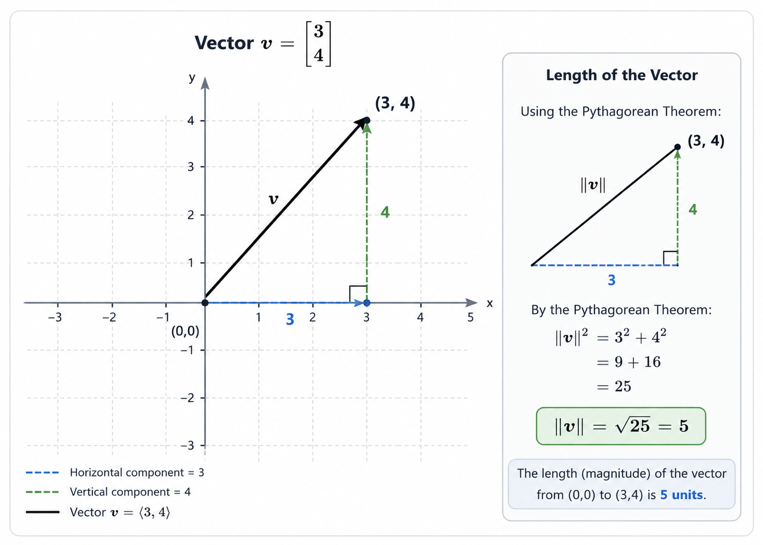
By the Pythagorean theorem,
\[\|\mathbf{v}\|^2=3^2+4^2.\]Therefore,
\[\|\mathbf{v}\| = \sqrt{3^2+4^2} = 5.\]The symbol
\[\|\mathbf{v}\|\]means the magnitude or length of the vector.
For a vector in $\mathbb R^2$,
\[\|\mathbf{v}\| = \sqrt{x^2+y^2}\]9. Direction matters too
Two vectors can have the same magnitude but point in different directions.
For example,
\[\mathbf{u} = \begin{bmatrix} 3\\ 4 \end{bmatrix}\]has magnitude $5$.
But
\[\mathbf{v} = \begin{bmatrix} -3\\ 4 \end{bmatrix}\]also has magnitude $5$:
\[\|\mathbf{v}\| = \sqrt{(-3)^2+4^2} = 5.\]Their lengths are the same, but their directions are different.
This is why a vector is more than simply a number representing distance.
10. From $\mathbb R^2$ to $\mathbb R^3$
So far, every vector we’ve seen has had two components.
For example,
\[\begin{bmatrix} 3\\ 2 \end{bmatrix}.\]We call these vectors two-dimensional vectors.
They live in
\[\mathbb R^2.\]The symbol $\mathbb R$ means the set of real numbers.
The $2$ tells us that there are two components.
Now imagine that we need one more direction.
For example, in three-dimensional space we might have
\[\mathbf{v} = \begin{bmatrix} 3\\ 2\\ 4 \end{bmatrix}.\]This vector has three components:
\[3,\qquad 2,\qquad 4.\]We say
\[\mathbf{v}\in\mathbb R^3.\]Now the components describe movement in three coordinate directions.
11. What does $\mathbb R^n$ mean?
We can continue this pattern.
A vector with:
- 2 components belongs to $\mathbb R^2$;
- 3 components belongs to $\mathbb R^3$;
- 4 components belongs to $\mathbb R^4$;
- $n$ components belongs to $\mathbb R^n$.
A general vector in $\mathbb R^n$ looks like
There are $n$ real numbers:
\[v_1,v_2,\ldots,v_n.\]These are the components of the vector.
12. Why do we need $\mathbb R^n$?
We can easily draw a vector in $\mathbb R^2$.
We can also draw one in $\mathbb R^3$.
But what about
\[\mathbb R^{10}\]or
\[\mathbb R^{100}?\]We cannot visualize these spaces in the same way.
But mathematically, there is no problem.
For example,
It is simply a vector with ten real components.
The important transition is this:
We began by thinking of vectors as arrows in two dimensions. Now we can think of a vector more generally as an ordered list of numbers.
That is the idea that allows linear algebra to work in very high dimensions.
13. Adding vectors in $\mathbb R^n$
The rule we learned in $\mathbb R^2$ does not change.
Suppose
Then
We simply add corresponding components.
For example,
\[\begin{bmatrix} 2\\ 1\\ 4 \end{bmatrix} + \begin{bmatrix} 3\\ -2\\ 1 \end{bmatrix} = \begin{bmatrix} 5\\ -1\\ 5 \end{bmatrix}.\]The same rule works whether the vector has $2$, $3$, or $100$ components.
14. Scalar multiplication in $\mathbb R^n$
Likewise, scalar multiplication works exactly as before.
For
and scalar $c$,
Again, nothing fundamentally changes.
We simply have more components.
15. Length in $\mathbb R^n$
The Pythagorean idea also extends naturally.
For
the length of the vector is
This is called the Euclidean norm.
For example,
\[\mathbf{v} = \begin{bmatrix} 1\\ 2\\ 2 \end{bmatrix}\]has length
\[\|\mathbf{v}\| = \sqrt{1^2+2^2+2^2} = \sqrt{9} = 3.\]So
\[\boxed{\|\mathbf v\|=3}.\]16. The zero vector
There is one particularly important vector:
the vector whose every component is zero.
In $\mathbb R^2$,
\[\mathbf 0= \begin{bmatrix} 0\\ 0 \end{bmatrix}.\]In $\mathbb R^3$,
\[\mathbf 0= \begin{bmatrix} 0\\ 0\\ 0 \end{bmatrix}.\]And in $\mathbb R^n$,
This is called the zero vector.
It behaves like the number zero:
\[\mathbf v+\mathbf 0=\mathbf v.\]17. The standard basis vectors
Now we can introduce another important idea.
In $\mathbb R^2$, consider
\[\mathbf e_1= \begin{bmatrix} 1\\ 0 \end{bmatrix}\]and
\[\mathbf e_2= \begin{bmatrix} 0\\ 1 \end{bmatrix}.\]These are called the standard basis vectors.
Why are they useful?
Because we can build every vector in $\mathbb R^2$ from them.
For example,
\[\begin{bmatrix} 5\\ 3 \end{bmatrix} = 5 \begin{bmatrix} 1\\ 0 \end{bmatrix} + 3 \begin{bmatrix} 0\\ 1 \end{bmatrix}.\]Therefore,
\[\begin{bmatrix} 5\\ 3 \end{bmatrix} = 5\mathbf e_1+3\mathbf e_2.\]We have just combined two vectors using scalar multiplication and addition.
That gives us our first glimpse of a linear combination.
We will study this idea carefully in the next chapter.
18. Standard basis in $\mathbb R^n$
The same idea works in $\mathbb R^n$.
There are $n$ standard basis vectors:
Every vector in $\mathbb R^n$ can be written as
This is an important idea.
A vector is not something mysterious.
It can be built by taking the standard directions and scaling them appropriately.
19. Connection with matrices
Now we can connect vectors back to the matrix equations we studied earlier.
Suppose
\[A= \begin{bmatrix} 2&1\\ 4&3 \end{bmatrix}\]and
\[\mathbf{x} = \begin{bmatrix} x_1\\ x_2 \end{bmatrix}.\]Then
The columns of $A$ are
\[\mathbf a_1= \begin{bmatrix} 2\\ 4 \end{bmatrix}, \qquad \mathbf a_2= \begin{bmatrix} 1\\ 3 \end{bmatrix}.\]Therefore,
So matrix-vector multiplication is actually a linear combination of the columns of the matrix.
This observation will become central in the next few chapters.
20. What have we learned?
Let’s pause before moving on.
We started with a simple movement:
\[3\text{ units right},\qquad 2\text{ units up}.\]We represented it as
\[\mathbf v= \begin{bmatrix} 3\\ 2 \end{bmatrix}.\]Then we learned that vectors have:
- components;
- magnitude;
- direction.
We learned how to:
- add vectors;
- multiply vectors by scalars;
- calculate their length;
- work with vectors in $\mathbb R^2$, $\mathbb R^3$, and $\mathbb R^n$.
And we discovered that every vector can be built from standard basis vectors.
Most importantly, we saw that
\[A\mathbf x\]is a combination of the columns of $A$.
Now we are ready for the next question.
Try It Yourself
Consider
\[\mathbf a= \begin{bmatrix} 4\\ 3 \end{bmatrix}\]and
\[\mathbf b= \begin{bmatrix} 2\\ -1 \end{bmatrix}.\]Question 1
Calculate
\[\mathbf a+\mathbf b.\]Question 2
Calculate
\[2\mathbf a.\]Question 3
Calculate
\[\|\mathbf a\|.\]Question 4
Write $\mathbf a$ using the standard basis vectors $\mathbf e_1$ and $\mathbf e_2$.
Answers
Answer 1
\[\mathbf a+\mathbf b = \begin{bmatrix} 4\\ 3 \end{bmatrix} + \begin{bmatrix} 2\\ -1 \end{bmatrix} = \begin{bmatrix} 6\\ 2 \end{bmatrix}\]Answer 2
\[2\mathbf a = 2 \begin{bmatrix} 4\\ 3 \end{bmatrix} = \begin{bmatrix} 8\\ 6 \end{bmatrix}\]Answer 3
\[\|\mathbf a\| = \sqrt{4^2+3^2} = \sqrt{25} ={5}.\]Answer 4
Since
\[\mathbf e_1= \begin{bmatrix} 1\\ 0 \end{bmatrix}, \qquad \mathbf e_2= \begin{bmatrix} 0\\ 1 \end{bmatrix},\]we have
\[\mathbf a=4\mathbf e_1+3\mathbf e_2.\]What comes next?
We have now learned how to add vectors and multiply them by numbers.
That gives us a new possibility.
If we have vectors $\mathbf v_1,\mathbf v_2,\ldots,\mathbf v_k$, we can form
\[c_1\mathbf v_1+ c_2\mathbf v_2+ \cdots+ c_k\mathbf v_k.\]This is called a linear combination.
But an even more interesting question is:
What collection of vectors can we create using all possible linear combinations?
That leads us to span.
And once we understand span, we can ask whether some of our vectors are redundant.
That leads us to linear independence.
So the next sequence is:
\[\boxed{ \text{Linear Combinations} \rightarrow \text{Span} \rightarrow \text{Linear Independence} }\]