Where are we going?
In the previous lesson, we learned that vectors can be:
- added together;
- multiplied by scalars;
- represented geometrically as arrows.
We also saw that the standard basis vectors can be used to construct other vectors.
For example,
\[\begin{bmatrix} 5\\ 3 \end{bmatrix} = 5 \begin{bmatrix} 1\\ 0 \end{bmatrix} + 3 \begin{bmatrix} 0\\ 1 \end{bmatrix}.\]We are now going to give this idea a name.
The expression
\[5 \begin{bmatrix} 1\\ 0 \end{bmatrix} + 3 \begin{bmatrix} 0\\ 1 \end{bmatrix}\]is a linear combination.
But this immediately raises a more interesting question:
If we are given some vectors, what other vectors can we create from them?
That question leads us to span.
1. What is a linear combination?
Suppose we have two vectors
\[\mathbf u = \begin{bmatrix} 2\\ 1 \end{bmatrix}\]and
\[\mathbf v = \begin{bmatrix} -1\\ 2 \end{bmatrix}.\]We can multiply them by numbers.
For example,
\[3\mathbf u\]and
\[2\mathbf v.\]We can then add the results:
\[3\mathbf u+2\mathbf v.\]This gives
\[3 \begin{bmatrix} 2\\ 1 \end{bmatrix} + 2 \begin{bmatrix} -1\\ 2 \end{bmatrix}.\]Calculate each part:
\[3 \begin{bmatrix} 2\\ 1 \end{bmatrix} = \begin{bmatrix} 6\\ 3 \end{bmatrix}\]and
\[2 \begin{bmatrix} -1\\ 2 \end{bmatrix} = \begin{bmatrix} -2\\ 4 \end{bmatrix}.\]Therefore,
\[3\mathbf u+2\mathbf v = \begin{bmatrix} 6\\ 3 \end{bmatrix} + \begin{bmatrix} -2\\ 4 \end{bmatrix} = \begin{bmatrix} 4\\ 7 \end{bmatrix}.\]So we have created the vector
\[\begin{bmatrix} 4\\ 7 \end{bmatrix}\]from $\mathbf u$ and $\mathbf v$.
This is a linear combination.
2. The general idea
Suppose we have vectors
\[\mathbf v_1,\mathbf v_2,\ldots,\mathbf v_k.\]We can multiply each vector by a scalar and add the results:
where
\[c_1,c_2,\ldots,c_k\]are scalars.
This expression is called a linear combination of the vectors.
The numbers $c_1,c_2,\ldots,c_k$ are called the coefficients.
For example,
\[2\mathbf v_1-3\mathbf v_2\]is a linear combination of $\mathbf v_1$ and $\mathbf v_2$.
So is
\[7\mathbf v_1+5\mathbf v_2.\]So is
\[0\mathbf v_1+4\mathbf v_2.\]The coefficients can be any real numbers.
3. Let’s see it geometrically
Take
\[\mathbf u= \begin{bmatrix} 2\\ 1 \end{bmatrix}\]and
\[\mathbf v= \begin{bmatrix} -1\\ 2 \end{bmatrix}.\]Suppose we want to form
\[\mathbf w=2\mathbf u+\mathbf v.\]The two scaled vectors are
\[2\mathbf u = \begin{bmatrix} 4\\ 2 \end{bmatrix}\]and
\[\mathbf v = \begin{bmatrix} -1\\ 2 \end{bmatrix}.\]Therefore,
\[\mathbf w = \begin{bmatrix} 4\\ 2 \end{bmatrix} + \begin{bmatrix} -1\\ 2 \end{bmatrix} = \begin{bmatrix} 3\\ 4 \end{bmatrix}.\]The geometry is important here.
We are:
- taking $\mathbf u$;
- stretching it by a factor of $2$;
- taking $\mathbf v$;
- adding the two resulting vectors.
The picture helps us see what the algebra is doing.
The final vector is the resultant of the two scaled vectors.
4. One vector can generate many vectors
Let’s start with just one vector:
\[\mathbf v= \begin{bmatrix} 2\\ 1 \end{bmatrix}.\]We can multiply it by any real number.
For example,
\[2\mathbf v = \begin{bmatrix} 4\\ 2 \end{bmatrix},\] \[3\mathbf v = \begin{bmatrix} 6\\ 3 \end{bmatrix},\]and
\[-2\mathbf v = \begin{bmatrix} -4\\ -2 \end{bmatrix}.\]We can also use fractions:
\[\frac12\mathbf v = \begin{bmatrix} 1\\ \frac12 \end{bmatrix}.\]So one vector can generate many other vectors.
But notice something interesting.
All of these vectors lie on the same line.
The vector
\[\begin{bmatrix} 2\\ 1 \end{bmatrix}\]points in one direction.
Multiplying it by a positive number makes it longer.
Multiplying it by a negative number reverses its direction.
Multiplying it by zero gives the zero vector.
So all scalar multiples of $\mathbf v$ lie along one line through the origin.
5. The span of one vector
This collection of all scalar multiples has a special name.
The span of $\mathbf v$ is the set of all vectors that can be obtained by multiplying $\mathbf v$ by a scalar.
In symbols,
\[\boxed{ \operatorname{span}\{\mathbf v\} = \{c\mathbf v:c\in\mathbb R\} }\]For
\[\mathbf v= \begin{bmatrix} 2\\ 1 \end{bmatrix},\]we have
\[\operatorname{span}\{\mathbf v\} = \left\{ c \begin{bmatrix} 2\\ 1 \end{bmatrix} : c\in\mathbb R \right\}.\]Geometrically, this is a line through the origin.
We can write that line as
\[y=\frac12x.\]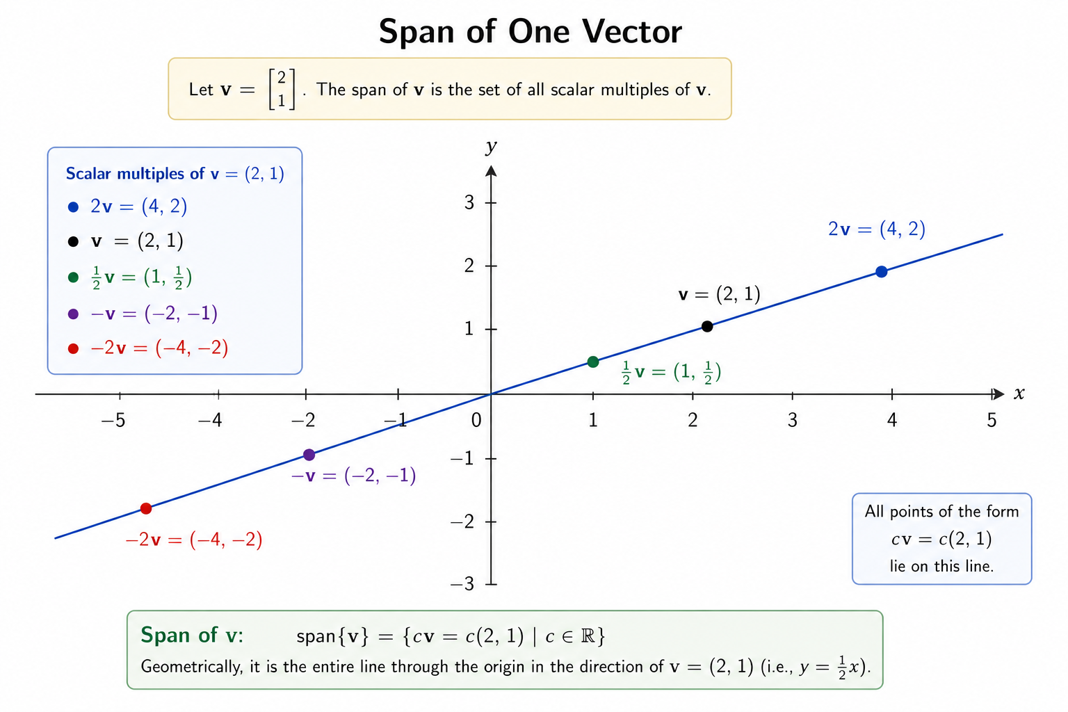
So:
The span of one nonzero vector in $\mathbb R^2$ is a line through the origin.
This is our first geometric interpretation of span.
6. Why does the line pass through the origin?
This is worth understanding.
Every vector in the span has the form
\[c\mathbf v.\]What happens if
\[c=0?\]Then
\[0\mathbf v=\mathbf 0.\]Therefore the zero vector is always in the span.
Since the zero vector is the origin, the line must pass through the origin.
This is why the span of a single nonzero vector is not an arbitrary line.
It is always a line through the origin.
7. What happens with two vectors?
Now let’s return to
\[\mathbf u= \begin{bmatrix} 2\\ 1 \end{bmatrix}\]and
\[\mathbf v= \begin{bmatrix} -1\\ 2 \end{bmatrix}.\]With one vector, we could move only along one line.
But now we have two different directions.
We can form
\[a\mathbf u+b\mathbf v\]for any real numbers $a$ and $b$.
For example,
\[\mathbf u+\mathbf v = \begin{bmatrix} 2\\ 1 \end{bmatrix} + \begin{bmatrix} -1\\ 2 \end{bmatrix} = \begin{bmatrix} 1\\ 3 \end{bmatrix}.\]Or
\[2\mathbf u-\mathbf v = 2 \begin{bmatrix} 2\\ 1 \end{bmatrix} - \begin{bmatrix} -1\\ 2 \end{bmatrix} = \begin{bmatrix} 4\\ 2 \end{bmatrix} - \begin{bmatrix} -1\\ 2 \end{bmatrix} = \begin{bmatrix} 5\\ 0 \end{bmatrix}\]We can keep changing $a$ and $b$.
This gives us many possible vectors.
The natural question is:
What is the complete collection of vectors we can create?
8. The span of two vectors
The span of $\mathbf u$ and $\mathbf v$ is the collection of all possible linear combinations of the two vectors.
In symbols,
Notice the difference.
For one vector:
\[c\mathbf v.\]For two vectors:
\[a\mathbf u+b\mathbf v.\]We allow the coefficients to take any real values.
9. What does this span look like?
For our vectors
\[\mathbf u= \begin{bmatrix} 2\\ 1 \end{bmatrix}, \qquad \mathbf v= \begin{bmatrix} -1\\ 2 \end{bmatrix},\]consider
\[a\mathbf u+b\mathbf v.\]Substituting,
\[a \begin{bmatrix} 2\\ 1 \end{bmatrix} + b \begin{bmatrix} -1\\ 2 \end{bmatrix} = \begin{bmatrix} 2a\\ a \end{bmatrix} + \begin{bmatrix} -b\\ 2b \end{bmatrix}\]Therefore,
As $a$ and $b$ vary over all real numbers, we obtain different points in the plane.
In this particular case, the two vectors point in genuinely different directions.
Their span fills the entire plane $\mathbb R^2$.
So:
\[\operatorname{span}\{\mathbf u,\mathbf v\} = \mathbb R^2\]Move the sliders to see how changing \(a\) and \(b\) changes the linear combination.
10. Why do two vectors fill the plane?
Think about the geometry.
One vector gives us only one direction.
So its scalar multiples trace out a line.
But two vectors pointing in different directions give us two independent directions of movement.
We can move:
- forward or backward in the direction of $\mathbf u$;
- forward or backward in the direction of $\mathbf v$.
By combining these movements, we can reach any point in the plane.
That is why the span becomes the whole $\mathbb R^2$.
This idea will become extremely important when we study linear independence.
11. Not every pair of vectors fills the plane
There is an important qualification.
Suppose
\[\mathbf u= \begin{bmatrix} 1\\ 2 \end{bmatrix}\]and
\[\mathbf v= \begin{bmatrix} 2\\ 4 \end{bmatrix}.\]Notice that
\[\mathbf v=2\mathbf u.\]So $\mathbf v$ does not give us a new direction.
It is simply a longer version of $\mathbf u$.
Therefore, every combination
\[a\mathbf u+b\mathbf v\]is really just a multiple of $\mathbf u$.
Indeed,
\[a\mathbf u+b\mathbf v = a\mathbf u+b(2\mathbf u)\]$$
(a+2b)\mathbf u. $$
So
\[\operatorname{span}\{\mathbf u,\mathbf v\} = \operatorname{span}\{\mathbf u\}.\]The span is still just a line.
This is a very important observation:
Adding another vector does not necessarily give us another direction.
12. A useful comparison
Consider these two cases.
Case 1: Same direction
\[\mathbf u= \begin{bmatrix} 1\\ 2 \end{bmatrix}, \qquad \mathbf v= \begin{bmatrix} 2\\ 4 \end{bmatrix}.\]Since
\[\mathbf v=2\mathbf u,\]their span is a line.
Case 2: Different directions
\[\mathbf u= \begin{bmatrix} 1\\ 2 \end{bmatrix}, \qquad \mathbf v= \begin{bmatrix} 2\\ -1 \end{bmatrix}.\]Neither vector is a scalar multiple of the other.
Together, they give two directions.
Their span is the whole plane:
\[\operatorname{span}\{\mathbf u,\mathbf v\} = \mathbb R^2.\]We will study the difference between these two situations carefully in the next lesson.
13. Linear combination versus span
These two ideas are closely related, but they are not the same thing.
Suppose
\[\mathbf u= \begin{bmatrix} 2\\ 1 \end{bmatrix}\]and
\[\mathbf v= \begin{bmatrix} -1\\ 2 \end{bmatrix}.\]The expression
\[3\mathbf u+2\mathbf v\]is one linear combination.
It gives us one vector:
\[3\mathbf u+2\mathbf v = \begin{bmatrix} 4\\ 7 \end{bmatrix}.\]But
\[\operatorname{span}\{\mathbf u,\mathbf v\}\]is the collection of every possible linear combination.
So:
A linear combination is one particular construction.
The span is the entire collection of vectors that can be constructed.
That distinction is fundamental.
14. Span is a set
It is useful to think of span as a set.
For one vector,
\[\operatorname{span}\{\mathbf v\}\]is the set
\[\{c\mathbf v:c\in\mathbb R\}.\]For two vectors,
\[\operatorname{span}\{\mathbf u,\mathbf v\}\]is the set
\[\{a\mathbf u+b\mathbf v:a,b\in\mathbb R\}.\]So when we say
\[\operatorname{span}\{\mathbf u,\mathbf v\} = \mathbb R^2,\]we are saying:
Every vector in $\mathbb R^2$ can be written as a linear combination of $\mathbf u$ and $\mathbf v$.
That is a much stronger statement than saying that we can produce one particular vector.
15. Span and the standard basis
We already encountered the standard basis:
\[\mathbf e_1= \begin{bmatrix} 1\\ 0 \end{bmatrix}, \qquad \mathbf e_2= \begin{bmatrix} 0\\ 1 \end{bmatrix}.\]Take any vector
\[\mathbf x= \begin{bmatrix} x_1\\ x_2 \end{bmatrix}.\]We can write
\[\mathbf x = x_1\mathbf e_1+x_2\mathbf e_2.\]Therefore every vector in $\mathbb R^2$ is a linear combination of $\mathbf e_1$ and $\mathbf e_2$.
Hence,
\[\operatorname{span}\{\mathbf e_1,\mathbf e_2\} = \mathbb R^2\]This is why the standard basis is so useful.
16. What about $\mathbb R^3$?
The same idea continues into three dimensions.
Consider
\[\mathbf e_1= \begin{bmatrix} 1\\ 0\\ 0 \end{bmatrix}, \qquad \mathbf e_2= \begin{bmatrix} 0\\ 1\\ 0 \end{bmatrix}, \qquad \mathbf e_3= \begin{bmatrix} 0\\ 0\\ 1 \end{bmatrix}.\]Take any vector
We can write
Therefore,
\[\operatorname{span} \{\mathbf e_1,\mathbf e_2,\mathbf e_3\} = \mathbb R^3\]The three standard basis vectors provide three directions.
17. The general idea in $\mathbb R^n$
Now we can finally state the general definition.
Suppose we have $k$ vectors
\[\mathbf v_1,\mathbf v_2,\ldots,\mathbf v_k \in\mathbb R^n.\]Their span is the set of all linear combinations:
This definition looks more abstract.
But the underlying idea is exactly the same:
Take the vectors, scale them however you want, and add them together. The collection of everything you can create is their span.
18. A geometric way to remember span
It helps to remember the following picture.
One nonzero vector
One direction:
\[\text{span}=\text{line}\]Two suitable vectors in $\mathbb R^2$
Two directions:
\[\text{span}=\text{plane}\]Three suitable vectors in $\mathbb R^3$
Three directions:
\[\text{span}=\mathbb R^3\]The word suitable matters.
If the vectors are redundant and point in directions already provided by the others, the span does not become larger.
19. Connection to matrix multiplication
Now let’s connect this to something we have already studied.
Suppose
\[A= \begin{bmatrix} 2&-1\\ 1&2 \end{bmatrix}.\]The columns of $A$ are
\[\mathbf a_1= \begin{bmatrix} 2\\ 1 \end{bmatrix}, \qquad \mathbf a_2= \begin{bmatrix} -1\\ 2 \end{bmatrix}.\]Now take
\[\mathbf x= \begin{bmatrix} x_1\\ x_2 \end{bmatrix}.\]Then
But matrix multiplication gives
Therefore,
\[A\mathbf x = x_1\mathbf a_1+x_2\mathbf a_2\]This is a linear combination of the columns of $A$.
And because $x_1$ and $x_2$ can be any real numbers,
\[A\mathbf x\]can produce every vector in
\[\operatorname{span}\{\mathbf a_1,\mathbf a_2\}.\]So the set of all possible outputs of $A\mathbf x$ is exactly the span of the columns of $A$.
This is a major connection between vectors and matrices.
20. Why this matters for $A\mathbf x=\mathbf b$
Earlier, we studied the equation
\[A\mathbf x=\mathbf b.\]Now we can look at it differently.
Because
\[A\mathbf x\]is a linear combination of the columns of $A$, the equation
\[A\mathbf x=\mathbf b\]is asking:
Can $\mathbf b$ be constructed as a linear combination of the columns of $A$?
In other words,
\[A\mathbf x=\mathbf b\]has a solution precisely when
\[\mathbf b\]belongs to the span of the columns of $A$.
This gives us a completely new way to think about systems of equations.
Instead of only thinking about rows and elimination, we can think geometrically about columns and span.
21. A simple example
Consider
\[A= \begin{bmatrix} 1&2\\ 2&4 \end{bmatrix}.\]Its columns are
\[\mathbf a_1= \begin{bmatrix} 1\\ 2 \end{bmatrix}\]and
\[\mathbf a_2= \begin{bmatrix} 2\\ 4 \end{bmatrix}.\]But
\[\mathbf a_2=2\mathbf a_1.\]Therefore the two columns point in the same direction.
Their span is only a line:
\[\operatorname{span}\{\mathbf a_1,\mathbf a_2\} = \operatorname{span}\{\mathbf a_1\}.\]Now consider the system
\[A\mathbf x= \begin{bmatrix} 3\\ 6 \end{bmatrix}.\]The right-hand side is
\[\begin{bmatrix} 3\\ 6 \end{bmatrix} = 3 \begin{bmatrix} 1\\ 2 \end{bmatrix}.\]Therefore it belongs to the column span.
So the system has a solution.
But consider
\[A\mathbf x= \begin{bmatrix} 3\\ 5 \end{bmatrix}.\]The vector
\[\begin{bmatrix} 3\\ 5 \end{bmatrix}\]does not lie on the line spanned by
\[\begin{bmatrix} 1\\ 2 \end{bmatrix}.\]Therefore it cannot be produced by any linear combination of the columns.
So this system has no solution.
22. The big picture
We can now connect several ideas we have learned.
A matrix has columns.
Those columns are vectors.
We can multiply those vectors by numbers and add them.
That gives us linear combinations.
All possible linear combinations form the column space, or span of the columns.
And therefore:
\[\boxed{ A\mathbf x = \text{a linear combination of the columns of }A }\]and
\[A\mathbf x=\mathbf b \quad\Longleftrightarrow\quad \mathbf b \text{ is in the span of the columns of }A\]when we are asking whether at least one solution exists.
This is the bridge from solving equations to understanding vector spaces.
Try It Yourself
Consider
\[\mathbf u= \begin{bmatrix} 1\\ 2 \end{bmatrix}, \qquad \mathbf v= \begin{bmatrix} 2\\ 1 \end{bmatrix}.\]Question 1
Calculate
\[2\mathbf u+3\mathbf v.\]Question 2
Is
\[\begin{bmatrix} 8\\ 7 \end{bmatrix}\]a linear combination of $\mathbf u$ and $\mathbf v$?
In other words, can we find $a$ and $b$ such that
\[a\mathbf u+b\mathbf v = \begin{bmatrix} 8\\ 7 \end{bmatrix}?\]Question 3
Consider
\[\mathbf w= \begin{bmatrix} 2\\ 4 \end{bmatrix}.\]Is $\mathbf w$ in
\[\operatorname{span}\{\mathbf u\}?\]Question 4
What is
\[\operatorname{span} \left\{ \begin{bmatrix} 1\\ 0 \end{bmatrix}, \begin{bmatrix} 0\\ 1 \end{bmatrix} \right\}?\]Answers
Answer 1
We have
\[2\mathbf u = 2 \begin{bmatrix} 1\\ 2 \end{bmatrix} = \begin{bmatrix} 2\\ 4 \end{bmatrix}\]and
\[3\mathbf v = 3 \begin{bmatrix} 2\\ 1 \end{bmatrix} = \begin{bmatrix} 6\\ 3 \end{bmatrix}.\]Therefore,
\[2\mathbf u+3\mathbf v = \begin{bmatrix} 2\\ 4 \end{bmatrix} + \begin{bmatrix} 6\\ 3 \end{bmatrix} = \begin{bmatrix} 8\\ 7 \end{bmatrix}\]So the vector is indeed a linear combination.
Answer 2
We want
\[a \begin{bmatrix} 1\\ 2 \end{bmatrix} + b \begin{bmatrix} 2\\ 1 \end{bmatrix} = \begin{bmatrix} 8\\ 7 \end{bmatrix}.\]This gives
\[a+2b=8\]and
\[2a+b=7.\]From the first equation,
\[a=8-2b.\]Substitute into the second:
\[2(8-2b)+b=7.\]Therefore,
\[16-4b+b=7\]so
\[-3b=-9\]and
\[b=3.\]Then
\[a=8-2(3)=2.\]Therefore,
\[\begin{bmatrix} 8\\ 7 \end{bmatrix} = 2\mathbf u+3\mathbf v\]So yes, it belongs to the span.
Answer 3
We have
\[\mathbf u= \begin{bmatrix} 1\\ 2 \end{bmatrix}.\]We want to know whether
\[\mathbf w= \begin{bmatrix} 2\\ 4 \end{bmatrix}\]is a scalar multiple of $\mathbf u$.
Indeed,
\[\mathbf w = 2 \begin{bmatrix} 1\\ 2 \end{bmatrix}.\]Therefore,
\[\mathbf w\in\operatorname{span}\{\mathbf u\}\]Answer 4
The two vectors are
\[\mathbf e_1= \begin{bmatrix} 1\\ 0 \end{bmatrix}, \qquad \mathbf e_2= \begin{bmatrix} 0\\ 1 \end{bmatrix}.\]Every vector
\[\begin{bmatrix} x\\ y \end{bmatrix}\]can be written as
\[x\mathbf e_1+y\mathbf e_2.\]Therefore,
\[\operatorname{span}\{\mathbf e_1,\mathbf e_2\} = \mathbb R^2\]The main idea to remember
There are three ideas to keep separate.
Linear combination
One particular combination:
\[c_1\mathbf v_1+\cdots+c_k\mathbf v_k.\]Span
All possible linear combinations:
Geometry
The span tells us what region of space those vectors can reach.
For example:
\[\text{one direction} \rightarrow \text{line}\]and
\[\text{two suitable directions in }\mathbb R^2 \rightarrow \text{whole plane}\]This geometric interpretation is the key.
What comes next?
We have seen that adding more vectors does not necessarily give us more directions.
For example,
\[\begin{bmatrix} 2\\ 4 \end{bmatrix} = 2 \begin{bmatrix} 1\\ 2 \end{bmatrix}.\]The second vector did not add anything new.
It was already contained in the direction of the first vector.
This raises a natural question:
When does a collection of vectors contain redundant information?
And more importantly:
When are vectors genuinely independent of one another?
That leads us to our next idea:
\[\text{Linear Independence}\]Before moving there, we will use what we have learned about span to understand exactly what it means for one vector to be redundant.